Now let's describe the double slit
experiment mathematically. The double slit experiment shows us that the total probability amplitude
is more than the sum of the individual amplitudes for both way 1 and 2.
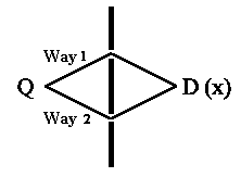 |
More precisely, the amplitude for way 1 consists of a path from source Q to slit 1 and then from slit 1 to detector D with coordinate x. We will designate each way using angle brackets
The total probability amplitude for both way 1 and 2 can be written:
| <x|Q> = <x|1><1|Q> + <x|2><2|Q> |
It's easy now to write the total probability amplitude for any
different way the system has gone from Q to x:
| <x|Q> = Σi=1<x|i><i|Q> |
Or we can just sum different paths of our system.
One can see from this expression that the right side corresponds to the left side if
we replace Σi=1 |i><i| by horizontal line | . Or it can be written
in mathematically:
| Σi=1 |i><i| = 1 |
This is pretty natural now using mathematical style. The above expression makes further mathematical derivations possible. Let's step back and analyze why it equals 1. We can calculate <x|1>, <x|2>, .... in a easier way than <x|Q>.
The qualities <1|Q> and <2|Q> show a fraction of source Q which makes a contribution from slit 1 and 2 into the probability amplitude. We can assign them in the following way a1 = <1|Q> and a2 = <2|Q>. If the source Q is situated directly in the middle between these two slits in our example then certainly a1 = a2 and the total probability amplitude <x|Q> is proportional to <x|1> + <x|2>. If we write <x|1>ºf1(x), <x|2>ºf2(x) and <x|Q>ºy(x) we come to well-known expression y(x) ~f1(x) + φ2(x).
In general, we obtain two identical ways of writing this mathematical
expression:
| <x|Q> = a1<x|1> + a2 <x|2> | y(x) = a1φ1(x) + a2φ2(x) |
Functions y(x) and φ(x) are called
wavefunctions. The form on the left was
created by Paul
Dirac and it has an advantage because "x" can be left:
| |Q> = a1 |1> + a2 |2> |
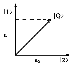 |
This equation is like vector |Q> that can be divided into two vectors |1> and |2>, where projection |Q> on direction |1> has length a1 and on direction |2> - a2. It's called left <| bra Vector and right |>ket vector.
If for instance we are interested in a momentum p rather than coordinate x then we just multiply it by <p| in the left side and obtain the probability amplitude for momentum p of a particle that comes from source Q:
<p|Q> = a1<p|1> + a2<p|2>
Now let's try to predict which way the particle will choose. In way 1 the total probability amplitude is as follows:
<x|Q> = a1<x|1> y(x) = a1φ1(x)
and the probability that it will be in a location with coordinate x:
| P1(x) = |a1|2 · |<x|1>|2 | P1(x) = |y(x)|2 = |a1|2 |φ1(x)|2 |
In order to obtain the square of this quantity we must multiply the probability
amplitude by complex conjugate quantity (for instance: |1 +
2i|2 = (1+2i)(1−2i) = 1−(2i)2 = 5).
When we want to write conjugate complex in a Dirac style we must just rotate brackets: (<x|1>)* = <1|x>.
P(x) is the probability of
locating a particle in the coordinate x. If we try to locate the particle
after it passes through a slit, it doesn't matter where it goes. The following
must be true:
| P1 = |a1|2 |
because a1 gives us part of probability amplitude that corresponds
to slit 1. Hence it should be true:
| P1 = -∞ò¥P(x)dx =
|a1|2 Σx
|<x|1>|2 = |a1|2
Σx <1|x> <x|1> = 1 <1|1> = 1, where Σx |x><x| = 1 |
P1 = -∞ò¥P(x)dx =
|a1|2 ò|f1(x)|2dx =
|a1|2
-∞ò¥ |φ1(x)|2dx
= 1 |
I.e. the total sum of all x values is equal to 1 in the Dirac meaning. The expression <1|1> = 1 and correspondingly ò|f1(x)|2dx = 1 demonstrates that the particle must somewhere in the space.
The treatment above holds true for a particle that has passed
through slit 1 (way 1). It's also
true for a particle that has taken way 2:
| P2 = |a2|2 <2|2> = 1 where -∞ò¥ |φ2(x)|2dx = 1 |
The total probability P that particle has taken way 1 (with probability
P1) or way 2 (with probability P2) and is detected
somewhere at x should be 1 in the particle must take either way 1 or way 2. Hence: P1 + P2
= 1
| P1 + P2 = 1
|a1|2 + |a2|2 = 1 |
We can extend our last result to any number of ways and obtain the general
equation:
| Σi |ai|2 = 1 |
| <i|i> = 1 -∞ò¥ |φi(x)|2dx = 1 |
The coefficients ai show the contributions of each individual ways. If we imagine a similar experiment with three slits with the third slit located far away from the first two, it is clear that the third slit would have only a small contribution to our intensity distribution (particularly, in the direction between first two slits). In other words, we could have described our system by approximation a1<x|1> + a2<x|2> because the third term a3<x|3> is too small to give considerable contribution to the above-mentioned sum. For instance we could have supposed that 98% of all particles goes by way1 and 2 and only 2% goes by way 3 (49% + 49% + 2% = 100%), this means that ratio Way 3/Way 1 is the following 2/49 ≈ 0,04. Nevertheless, the ratio of probability amplitudes gives |a3|/|a1| ≈ 0,2, where |a1| = |a2| = 0,7 that's why |a3| ≈ 0,14.
Now let us carry out the two slit experiment and not concerned ourselves with which slits the particles pass through. The probability of detecting a particle in a location with coordinate x is as follows:
| P(x) = |<x|Q>|2
<x|Q> = a1<x|1> + a2<x|2> |
P(x) = |y(x)|2
y(x) = a1φ1(x) + a2φ2(x) |
| P(x) = |a1|2 |<x|1>|2 +|a2|2|<x|2>|2 + a1*a2<1|x><x|2> + a1a2*<2|x><x|1> | P(x) = |a1|2|φ1|2+|a2|2|φ2|2+a1*a2φ1*φ2 + a1a2*φ1φ2* |
The first two terms are similar to the probability that is obtained when one is interested in the a way particle has passed through slits. The last terms are interference terms; they describe the increase or decrease of intensity.
The total probability of detecting a particle is, as always, equal to 1:
1 = |a1|2∫|φ1|2dx + |a2|2∫|φ2|2dx + a1*a2òf1*φ2dx + a1a2*òf1φ2*dx
here ∫|φ1|2dx =
∫|φ2|2dx = 1
and |a1|2 + |a2|2 =
1 and hence one can obtain from the last:
| -∞∫+∞φ1*φ2dx = -∞∫+∞φ1φ2*dx = 0 |
In the Dirac style it means:
| <1|2> = <2|1> = 0 |
So, we can resume all our results for any amount of ways a particle can pass through the slits:
|
di,k = { | 1 for i = k | ||
| 0 for i ¹ k | ||||
One talks about orthonormal states which are similar to two normalized vectors i and k which are perpendicular to each other:
| i · k | = { | 1 for i = k |
| 0 for i
¹ k
|
![]()
Auf diesem Webangebot gilt die Datenschutzerklärung der TU Braunschweig mit Ausnahme der Abschnitte VI, VII und VIII.