Die sich aus den (1s)-Wellenfunktionen ergebenen Molekülorbitale
gemäß:
| y+ ~ (φA
+ φB)
y- ~ (φA - fB) |
sind im Folgenden als 3D- und als Konturplot dargestellt.
 |
 |
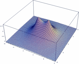
| Abb1 (a+b):Positive Linearkombination: y+ ~ (φA + φB); (b): Kontorplot | |
 |
 |
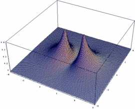
| Abb2 (a+b): Negative Linearkombination: y- ~ (φA - φB); (b): Konturplot | |
| |
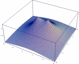
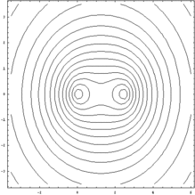
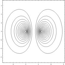
| Abb3 (a+b):Aufenthaltswahrscheinlichkeit; positive Linearkombination: |y+|2; (b): Konturplot | |
 |
 |
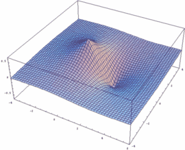
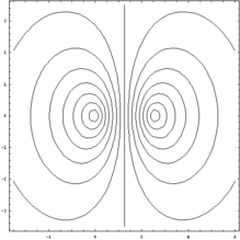
| Abb4 (a+b):Aufenthaltswahrscheinlichkeit; negative Linearkombination: |y-|2; (b): Konturplot | |
Mathematica-Besitzer können sich leicht selber die Funktionen darstellen:
Rgl=2.4;
psiP=Exp[-Sqrt[x^2+y^2]/2]+Exp[-Sqrt[(x-Rgl)^2+y^2]/2]
psiM=Exp[-Sqrt[x^2+y^2]/2]-Exp[-Sqrt[(x-Rgl)^2+y^2]/2]
Plot3D[psiM, {x,-4,6}, {y,-4,4},
PlotPoints -> 50, ImageSize ->500,
PlotRange -> All]
Plot3D[psiP, {x,-4,6}, {y,-4,4},
PlotPoints -> 50, ImageSize ->500,
PlotRange -> All]
Plot3D[psiP^2, {x,-4,6},
{y,-4,4}, PlotPoints -> 50, ImageSize ->500,
PlotRange -> All]
Plot3D[psiM^2, {x,-4,6},
{y,-4,4}, PlotPoints -> 80, ImageSize ->500,
PlotRange -> All]
ContourPlot[psiM,{x,-3.5,3.5+Rgl},{y,-3.5,3.5},PlotPoints ->50, ImageSize
->500, Contours -> 15, ContourShading -> False]
ContourPlot[psiP,{x,-3.5,3.5+Rgl},{y,-3.5,3.5},PlotPoints ->50,
ImageSize -> 500, Contours -> 15, ContourShading -> False]
ContourPlot[psiM^2,{x,-3.5,3.5+Rgl},{y,-3.5,3.5},PlotPoints ->50, ImageSize
->500, Contours -> 15, ContourShading -> False, PlotRange -> All]
ContourPlot[psiP^2,{x,-3.5,3.5+Rgl},{y,-3.5,3.5},PlotPoints ->50,
ImageSize -> 500, Contours -> 15, ContourShading -> False, PlotRange ->
All]
![]()
Auf diesem Webangebot gilt die Datenschutzerklärung der TU Braunschweig mit Ausnahme der Abschnitte VI, VII und VIII.