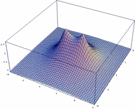
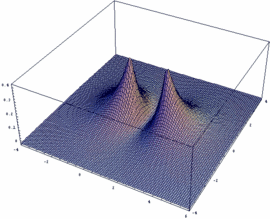
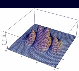
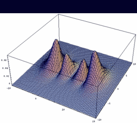
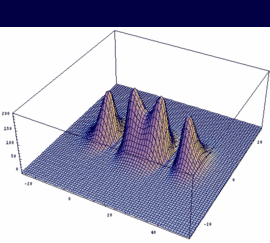
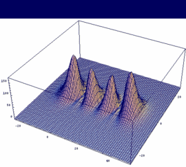
The following 3D plots are representations of molecular orbitals (MOs) based of atomic orbital (AO) wave functions. On the left side, the probability amplitude Ψ is plotted, on the right side the probability density |Ψ|2.
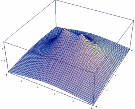 1σg = 1sA + 1sB bonding |
 |
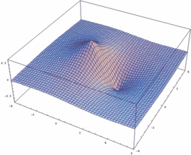 1σu = 1sA - 1sB antibonding |
 |
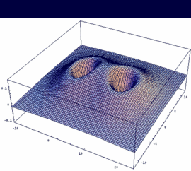 2sg = -[2sA + 2sB] bonding |
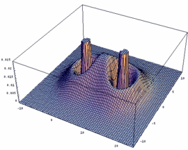 |
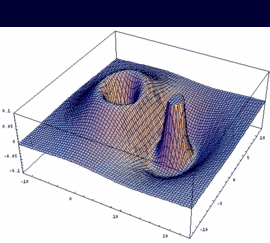 2su = -[2sA - 2sB] antibonding |
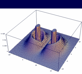 |
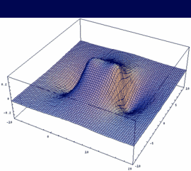 3σg = 2pzA - 2pzB bonding |
 |
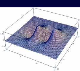 3su = 2pzA + 2pzB antibonding |
 |
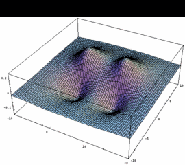 1pu = 2pxA + 2pxB bonding (dto. 2pyA+2pyB) |
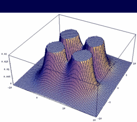 |
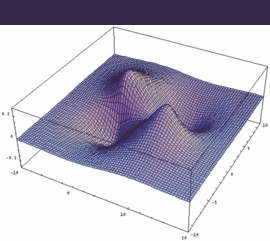 1pg = 2pxA - 2pxB antibonding (dto. 2pyA-2pyB) |
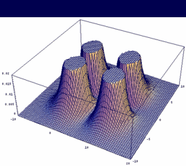 |
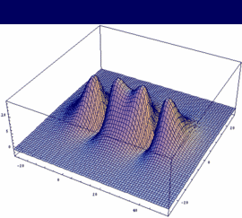 σg = -3dzA + 3dzB bonding |
 |
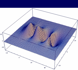 σu = -3dzA - 3dzB antibonding |
 |
The software "Mathematica" provides you easily with representations of MO functions.
The lines below illustrate a program for the calculation such functions. The variable Rgl (sensible choices for 1s and 2p are 2.3 and 12, respectively) represents the distance between the atoms and is one of the input items. In addition, the respective AO functions need to be defined (e.g. "psi=p2y[0]+p2y[Rgl]). The program below uses dz orbitals not normalized.
In our example, an overlap of two 3dz orbitals and 26 as internuclear distance is assumed.
"Graphische Darstellung der MO und deren Betragsquadrat"
"Internuklearer Abstand"
Rgl=26.0
r[zgl_]:=Sqrt[(z-zgl)^2+y^2]
s1[zgl_]:=2*Exp[-r[zgl]]
s2[zgl_]:=(2-r[zgl])*Exp[-r[zgl]/2]/Sqrt[8]
p2z[zgl_]:=Exp[-r[zgl]/2]*(z-zgl)/Sqrt[8]
p2y[xgl_]:=Exp[-r[zgl]/2]*y/Sqrt[8]
d3z[zgl_]:=Exp[-r[zgl]/3]*(2*r[zgl]-3*(z-zgl)^2)
psi=-d3z[0]+d3z[Rgl];
Plot3D[psi, {z,-Rgl,2*Rgl}, {y,-Rgl,Rgl}, PlotPoints
-> 70, PlotRange ->All, ImageSize ->500]
Plot3D[psi^2,{z,-Rgl,2*Rgl},{y,-Rgl,Rgl}, PlotPoints
-> 70, PlotRange ->All, ImageSize ->500]
![]()
Auf diesem Webangebot gilt die Datenschutzerklärung der TU Braunschweig mit Ausnahme der Abschnitte VI, VII und VIII.