![]()
Stationary perturbation theory is concerned with finding the changes in the discrete energy levels and the changes in the corresponding energy eigenfunctions of a system, when the Hamiltonian of a system is changed by a small amount. Let
H = H0 + H = H0 + λW
H0 is the unperturbed Hamiltonian whose eigenvalues E0p and eigenstates |φip> are known. LetH0 | φip> = E0p | φip >.
Here i denotes the degeneracy. Assume that the matrix elements of H in the eigenbasis of H0 are small compared to the matrix elements of H0.<φip|H ' |φip> << <φip | H0 | φip > = E0p.
We write
H = λW
with λ << 1 and <φip|W |φip> ≈ E0p.
![]()
Example:H = H0 + H
is the Hamiltonian of a perturbed one-dimensional harmonic oscillator.
|
![]()
We are looking for the eigenvalues
E(λ)
and the eigenstates |ψ(λ) >
of H(λ) = H0 + λW.
H |ψp> = Ep |ψp>. Since λW
is small, we assume that E and |ψ>
can be expanded as a power series in λ.
Ep=E0p+λE1p+λ2E2p+...,
We may then write
(H0 + λW)(|ψp0>+λ|ψp1> + λ2|ψp2> + ...)
=(E0p + λE1p + λ2E2p + ...)(|ψp0> + λ|ψp1> + λ2|ψp2 > +...). This equation is must be
valid over a continuous range of λ.
Therefore we equate coefficients of equal powers of λ
on both sides to obtain a series of equations that represent successively
higher orders of the perturbation.
(H0-E0p)|ψp0> = 0
implies that |ψp0> is a linear combination of unperturbed eigenfuctionns |φip>
with the corresponding eigenvalue E0. We choose
<ψp0|ψp0> = 1.
|ψps>
is not uniquely defined. We can add an arbitrary multiple of |ψp0>
to each |ψps>
without affecting the left hand side of the above equations. Most
often this multiple is chosen so that <ψp0|ψps>=0.
The perturbed ket is then not normalized. We then have
0
= To calculate the energy
to sth order, we only need to know the state vector to order s-1.
En=E0n+<φn|H|φn>+O(&lambda2) En = E0n + O(λ2).
To first order, the eigenvalues of H are equal to the eigenvalues
of the unperturbed Hamiltonian H0.
First-order eigenvector corrections:
(H0-E0p)| ψp1>
= (E1p-W)| ψp0 >
= (E1p-W)| φp >.
|ψp0> is an eigenstate of the unperturbed Hamiltonian. We may expand
in terms of the basis vectors
|φip' >.
In the expansion bp = 0 because <ψp0| ψpi > = 0.
Multiply from the left by
<φip'' |.
Therefore
Since we have found the
expression for the state vector to first order, we can now find the expression
for the energy to second order.
Let H = H0 + H = H0 + λW.
In practice, after having derived the perturbation expansion, we often set λ = 1 and let H = W be small.
The ground state is not degenerate. The potential energy of an electron outside a uniformly charged sphere of radius r0 and total charge qe
is Inside the sphere the potential
energy is From Gauss law we know
that Let
since r0 << a0,
=4⋅10-9eV.
A
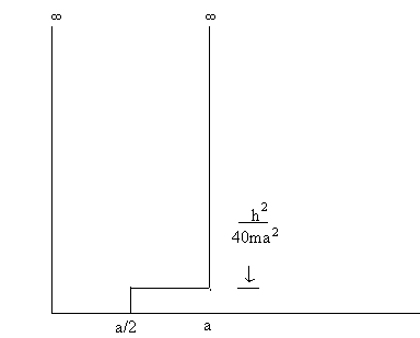
particle of mass m is in an infinite potential well perturbed as
shown in the figure.
(a)
Calculate the first-order energy shift of the nth eigenvalue due
to the perturbation.
(b)
Write out the first three non vanishing terms for the first-order perturbation
expansion of the ground state in terms of the unperturbed eigenfunctions
of the infinite well.
(c)
Calculate the second-order energy shift for the ground state.
H = H0 + H.
The eigenvalues of H0 are not degenerate.
The second-order energy shift of the ground state is always negative.
Auf diesem Webangebot gilt die Datenschutzerklärung der TU Braunschweig mit Ausnahme der Abschnitte VI, VII und VIII.
|ψp>=|ψp0>+λ|ψp1>+λ2|ψp2>+....
![]()
(H0-E0p)|ψp0>=0
![]()
(H0-E0p)|ψp1>=(E1p-W)|ψp0>
![]()
(H0-E0p)|ψp2>=(E1p-W)|ψp1>+E2p|ψp0>
![]()
(H0-E0p)|ψp3>=(E1p-W)|ψp2>+E2p|ψp1>+E3p|ψp0>
![]()
...
![]()
![]()
![]()
![]()
First-order
perturbation theory for non-degenerate
levels
Consider a particular non-degenerate
eigenvalue E0n of H0.
H0| φn> = E0n| φn>.
The other eigenvalues of H may or may not be degenerate. We
have | ψn0> = | φn>
and E1n = <φn |W| φn>. The first-order energy correction therefore is λE1n = < φn |H| φn>. We have ![]()
![]()
Example:
![]()
![]()
![]()
![]()
![]()
![]()
![]()
![]()
![]()
![]()
Example:
![]()
![]()
![]()
![]()
![]()
Second-order
perturbation theory for non-degenerate levels
Second-order
energy corrections:
![]()
![]()
![]()
![]()
Example:
![]()
![]()
![]()
![]()
![]()
Problems:
Calculate
the first-order shift in the ground state of the hydrogen atom caused by
the finite size of the proton. Assume the proton is a uniformly charged
sphere of radius r = 10-13cm. The ground state wave function
of the hydrogen atom is ![]() and
the Bohr constant is
and
the Bohr constant is
![]()
Solution:
![]()
![]()
![]() (SI
units).
(SI
units).
![]()
![]()
![]()
![]()
![]()
![]()
![]()
![]()
![]()
Solution:
![]()
![]()
![]()
![]()
(a)
![]()
![]()
![]()
(b)
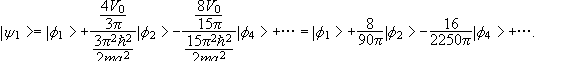
First-order perturbation theory yields
![]()
![]()
![]()
![]() if n is odd.
if n is odd.
![]()
![]()
![]()
(c)
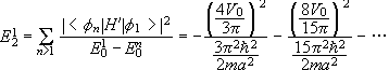
![]() second-order
energy shift for the ground state.
second-order
energy shift for the ground state.