Doppler Broadening

Another example of the inhomogeneous line broadening is so called Doppler broadening which is typical in gaseous samples. As known, the Doppler effect results in light frequency shift when the source is moving toward, or away from the observer. When a source emitting radiation with frequency $\nu_0$ moves with a speed $\textbf{v}$, the observer detects radiation with frequency:

$$\nu = \nu_0\left(1 \pm \frac{v_z}{c}\right),$$ (24)

where the sign $+$ and $-$ is related to an approaching and receding source, respectively.

Molecules in a gas chaotically move in all directions and the observer detects the corresponding Doppler-broadened spectral line profile. This profile reflects the distribution of molecular velocities along the line of detection, which we designate as $Z$ axis. In case of the thermal equilibrium this velocity distribution is known as Maxwell-Boltzmann distribution:

$$n(v_z)dv_z = \sqrt{\frac{2\, k\, T}{\pi\, m}}\,exp\left(-\frac{m\, v_z^2}{2\,k\,T}\right)$$ (25)

Here $n(v_z)dv_z$ is a relative number of atoms with the velocity component $v_z$ parallel to the light beam, $m$ is the particle mass, $k$ is the Boltzmann constant, and $T$ is the gas temperature.

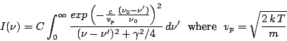
Combining eqs.(25) and (24), we can get the expression for the light intensity as function of $\nu$

$$I(\nu) = I_0 \sqrt{\frac{4\,ln 2}{\pi}}\frac{1}{\Delta\nu_D}... ...\nu_D = \frac{2\,\nu_0}{c} \,\sqrt{\frac{2\, ln 2\, k\, T}{m}}$$ (26)

The value $\Delta\nu_D$ (Doppler width) is the linewidth of the distribution at the half-hight. The distribution (26) is of the Gaussian type and it is called the Doppler profile.

It is seen that the Doppler width $\nu_D$ is proportional to the transition frequency $\nu_0$, to the square root of the gas temperature $T$, and inverse to the squire root of the particle mass. For transitions which belong to the visible or the near-UV spectral range when the gas temperature is around 300 K, the Doppler width is typically within one GHz. However, the hydrogen atoms and molecules has exceptionally high Doppler widths of around 30 GHz due to their low mass. For the visible part of the spectrum the Doppler line broadening is usually much larger than the lifetime broadening. Therefore, the experimentally obtained line profiles have usually the Gaussian shape. In contrast, for microwave transitions, or in conditions of high collisional broadening, the lifetime broadening becomes larger than the Doppler one resulting in the Lorentz-type line profiles.

In case $\delta\nu_L$ and $\delta\nu_D$ have have comparable amplitudes, the observed spectral line can be obtained by the convolution of the Gaussian and Lorentz profiles:

$$I(\nu) = C \int_0^\infty \frac{exp\left(-\frac{c}{v_p}\frac{... ...\nu' \:\:\:\mbox{where}\:\:\: v_p = \sqrt{\frac{2\, k\, T}{m}}$$ (27)

This intensity profile is called the Voigt profile. For example, Voigt profiles play an important role in the spectroscopy of stellar atmospheres where accurate measurements of line wings allow the contributions of Doppler broadening, or natural linewidth of collision line broadening to be separated. From this measurements the temperature and pressure of the emitting or absorbing layers in the stellar atmospheres can be determined.

Auf diesem Webangebot gilt die Datenschutzerklärung der TU Braunschweig mit Ausnahme der Abschnitte VI, VII und VIII.