We are already familiar with the measurement process required to determine "Which way a particle goes" in
the double slit experiment:
It should be possible to simultaneously
observe it pass through either slit 1 or 2. The probability amplitude y(x) = a1φ1(x) +
a2φ2(x) will change during measurements. It takes value
y(x) = a1φ1(x) if a particle pass
through slit 1 and it takes y(x) =
a2φ2(x) if a particle crosses slit 2. Therefore, the
wavefunction will also change during measurements (either
a1φ1(x) or a2φ2(x)). One can also describe the wavefunction as collapsing or the state
vector being reduced since the total amplitude a1|1> +
a2|2> is decreased either on a1|1> or
a2|2>. This means that when one makes "Which way a particle goes"
measurements, the sum is taken from the initial superposition (linear
combination) using measurements. After making measurements, the system is
described only with function φ1(x) (and
φ2(x) correspondingly). The a1 and
a2 values are just constants and they can be neglected. This
new function φ1(x) (and
f2(x) correspondingly) determines how the system develops successively. If you don't understand this, don't worry.
Nobody understands it, but it works! Only recently have scientists began to study
this "wavefunction collapse" intensely in order to better understand
the measurement principle in quantum mechanics. Now we shoulb be satisfied with saying that the "which way" measuring operation influences the
wavefunction in a way that φ1 or φ2 only stays and is the
system characteristics. So, the next step of the system is described by y = φ1 (and y =
φ2(x) correspondingly). Let's have a look at a simple experiment with
polarizers.
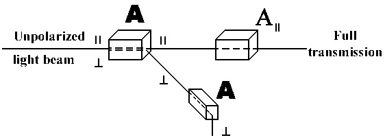
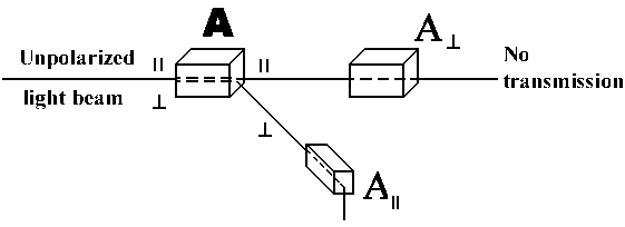
The unpolarized light beam Q is split by polarizer A into parallel (||) and perpendicular (^) components being || and ^ relative to the marked axis of A.
| |Q> = a|||A||> + a^|A^> |
There are two states of A: |A||> and |A^> that are detected by the analyzer. The state vector |Q> is then |Q> = a|||A||> + a^|A^>. For the total probability amplitude of parallel and perpendicular polarization (also called the sum of all possibilities) we have:
<Q|Q> = 1 = (a||*<A||| + a^*<A^|)·(a|||A||> + a^|A^>) = |a|||2<A|||A||> + a^*a||<A^|A||> + a||*a^<A|||A^> + |a^|2<A^|A^>
= |a|||2 + |a^|2 = 1
|a^|2 is the ^ polarization probability.
|a|||2 is the ||
polarization probability.
The analyzer A projects |Q> on the analyser states |A||> or |A^>. After being successively projected on, for instance, |A||> we will observe |A||> on the mounted A|| analyser and never |A^>. The system transmits only |A||> state and the probability amplitude should be equal only to a|||A||> now.
Measurement || : |<A|||Q>|2 = |a|||2
Measurement ^: |<A^|Q>|2 = |a^|2
After passing of analyser A it is |Q>new = a|||A||>. Each successive ideal analyser with the same qualities measures only ||
<A|||Q>new = a||<A|||A||> = a||
The observation probability is then as follows
P|| = |<A|||Q>new|2 = |a|||2
P^ = |<A^|Q>new|2 = 0
And also we can have a look to the projection on state A^> passing through one analyser:
|Q>new = a^|A^>
P^ = |<A^|Q>new|2 = |a^|2
P|| = |<A|||Q>new|2 = 0
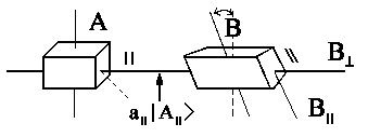
Let's now rotate second polarizer relatively to the first one. Since it is another analysing device we will call it B having the states |B||> and |B^>. The total probability amplitude B is equal to
|q> = b|||B||> + b^|B^>
We must always pay attention to the fact that || and ^ should be determined relative to polarizers! Let's observe the exit of A analyser, i.e. we initially have |Qnew> = a|||A||>.
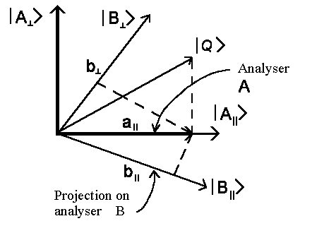 |
b|| is the component of |B||> state and b^ is the component of |B^> state. These components are defined by the projection of |q> vector on |B||> and |B^>-axis correspondingly. The "initial point" |Qnew> for the ||-channel is a|||A||> = b|||B||> + b^|B^> = |q>. Therefore the B|| measurement gives finally: <B|||Qnew> = a||<B|||A||> = b||<B|||B||> + b^<B|||B^>, and from this it's clearly (<B|||B||> = 1 und <B|||B^> = 0):
b|| = a||<B|||A||>
and
correspondingly: b^ = a||<B^|A||>
One follows <B|||A||>¹ 1 and <B^|A||>¹ 0, since B|| isn't parallel to A|| and B^ isn't perpendicular to A||.
Then we will have for the probability we will observe || polarized beam:
P|| = |b|||2 = |a|||2 |<B|||A||>|2
or for ^ :
P^ = |b^|2 = |a|||2 |<B^|A||>|2
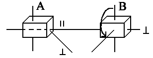 |
If the analyser B is rotated in a way that A||^ B||, then
one will have <B|||A||> = 0 and <B^|A||> = 1, i.e.
| P|| = 0 |
Now let us put the third analyser C between A and B in such a way that this one angle J takes 0° < J < 90° but it is still B ^ A.

In this arrangement, light comes from B^. If we put away C there is no light passing through B^! The particles (photons) after moving through analyser C possess a new state c||f|| + c^f^, having c|| or c^ which depends on the probability amplitude (as a function of rotation angle J). Now it's the initial state for all others successive measurements and hence there is also a component B^. However, the component B^ is zero without analyser C, because a vertical arrangement was chosen between A and B.
The measuring state is always defined relative to polarizer with which one
carries out the experiments. The probability amplitude projects A on state A|| (or
A^) (analyser A). Now the amplitude is
determined by state A|| (or A^). Now it's the initial point for
successive experiments. I.e. when measuring polarization with the rotated
polarizer C, we now study c|| and
c^ relative to this new polarizer C.
Certainly, we can measure other values as for instance the wavelength of the light without influence from the measurement
of the polarization.
If we make a measurement of the location, then we project y on the "place location" x and from now y corresponds to x. Now the next measurement of the momentum will give a different result than without the previous local measurement.
Now let's C will not be an analyser, but it will be a new instrumentation or a machine M which rotates polarization in any way. The light of particular state (|A||> or |A^>) then goes through this instrument M and finally we will have B state (|B||> or |B^> . Hence we write in a known way from right to left::
<after|instrument|before>
If we have the initial state |A||> and then try to make measurement after instrument M, we will have the following noting for the probability amplitude:
<B^|M|A||>
And if we have the initial state |A^> then we will have the following noting for the probability amplitude to detect photons:
<B^|M|A^>
which has another value than <B^|M|A||>. And finally the probability amplitude to detect a photon in state <B||| is as follows
<B|||M|A||> or <B|||M|A^>
Hence we have four possibilities:
after |
before | ||
| || | ^ | ||
| || | <B|||M|A||> | <B|||M|A^> | |
| ^ | <B^|M|A||> | <B^|M|A^> | |
And now let's try to write a more general equation for a photon state (which initially has had arbitrary state φ) that has just passed through instrument M. So, the instrument M somehow changes the polarization state of incident photon and therefore we will have another state y after the instrument:
y = Mφ
The symbol M is neither the probability amplitude nor state (nor vector). It's something new that is called the Operator. The operator acts upon the initial state φ and produces new state y. We will mark operators using bold letters. Sometimes they are marked by sign ^ above the letter of operator, for instance: Ô. Here you can find a bit more information about operators.
Everything is wonderful and good, however how will we write down amplitudes
and wavefunctions now?
There are three possibilities and they
are closely connected with the following people:
| 1) Matrix algebra | (Werner Heisenberg) | } | They are all equivalent in mathematical way |
| 2) Operators and ODE | (Erwin Schrödinger) | ||
| 3) Curve integral | (Richard Feynman) |
One can find out more details about Operators and the Schrödinger Differential equation in these two links.
![]()
Auf diesem Webangebot gilt die Datenschutzerklärung der TU Braunschweig mit Ausnahme der Abschnitte VI, VII und VIII.