Heteronuclear Molecules AB

As well for a treatment of heteronuclear molecules, the qualitative aspects of the LCAO method apply. To get a successful combination of the kind Ψ = c_AΦ_A + c_BΦ_B

• The energy levels of Φ_A and Φ_B of the single atoms A and B shall not differ too much. Therefore, the two atoms' valence orbitals combine strongly, whereas combinations between valence orbitals and inner shell orbitals are neglectable. The latter are of pronounced low energy.
• The product Φ_A·Φ_B shall be high, this is often referred to as "Principle of maximal overlap".
• The functions Φ_A and Φ_B must show the same symmetry with respect to the molecule's axis.

Let us apply the conditions for an effective linear combination of atomic orbitals to the hydrogene chloride molecule. The first condition, for which mathematical evidence will be delivered below, forbids combinations between a hydrogene AO and 1s-, 2s- and 2p-orbitals of of chlorine for these AOs (the 3s-orbital might be classified as a borderline case) are of too low energy. In contrast, the atomic orbitals 3p_x, 3p_y and 3p_z remain as candidates for combinations with the 1s-AO which is the orbital of lowest energy of the hydrogene atom. Taking symmetry into account, the 3p_z-AO of chlorine is the orbital that has to be introduced in an LCAO approach that shall describe HCl. As we will learn in one of the following chapters (Hybridization), the 3s-AO of Cl is to some degree involved in this combination, but this does not call the description presented here into question. From these considerations and from the building-up principle, the ground state of the hydrogene chloride molecule is:

(1s)² (2s)² (2p_z)² (2p_x)² (2p_y)² (3s)² (3p_x)² (3p_y)² {c_AH(1s) + c_BCl(3p_z)}²

Where the chlorine atomic orbitale are simply denoted as 1s, 2s, ... 3p_y. Though these orbitals do not contribute to bonding, they appear like MOs of related symmetry, i.e. the s- and p_z-orbitals as σ- and the p_x and p_y π-molecular orbitals. A σ-state represents the orbital emerging from the {c_AH(1s) + c_BCl(3p_z)}. The energy level of this MO is below the π-orbitals occupied by the (3p_x)and (3p_y) electrons of chlorine. With numbers added, the electronic configuration of the molecules is described as:

The relation between an orbital of the molecule AB in the LCAO approach and the atomic orbitals, i.e. the components for this approach (Φ_A and Φ_B) are worth being considered, especially in the case where this molecular orbital is occupied by electrons that can be regarded as valence electrons of the unbound atoms A and B. Assuming a possibility to separate the atoms that form molecule AB, we expect such electrons to appear again in the two atomic orbitals Φ_A and Φ_B. (We already encountered this aspect when treating the hydrogene cation). Thus, it is allowed to regard these electrons as originating from a Φ_A- or Φ_B-state, now sharing a state Ψ = c_AΦ_A + c_BΦ_B. Reversely, we are able to imagine the two atoms approaching each other without interaction and then pairing both electrons.When the molecule AB is formed, there is no possibility to discriminate between electron A and B, i.e. both belong to that AB molecule. In fact, this impossibility is the reason for a chemical bond.

Let us have a look on the mathematical treatment. For all relevant solutions of the secular equation for a heteronuclear molecule AB

c_A(α_A−E) + c_B(β − E·S) = 0
c_A(β − E·S) + c_B(α_B−E) = 0

the determinant becomes zero, i.e. the values for energy E accomplish equation

(α_A-E)(α_B-E) - (β-ES)² = 0

To avoid the effort of deriving the exact solution of this equation quadratic in E, we assume that the energies of the bonding MO and the lowest of the two AOs differ only slightly. In case that Φ_A is this AO, E ≈ α_A−ΔE reflects this assumption without further restrictions to the general applicability. The ΔE represents the shift in energy that corresponds with the bonding effect. Replacing E in the quadratic equation yields

(α_A - α_A+ ΔE)(α_B - α_A + ΔE) = (β - (α_A - ΔE)S)²

As ΔE << α_A, we can write

ΔE·(α_B - α_A) = (β - α_AS)²

ΔE = [ β - α_AS ]² / [ α_B-α_A ].

For the energy level for the bonding MO we get:

Ebonding =  αA- [ β - aAS ]² / [ αB - αA ]

In an analogous way, we derive the energy of the antibonding MO, starting with E ≈ α_B-ΔE.

(α_A - α_B+ ΔE)(α_B - α_B +ΔE) = (β - (α_B - ΔE) S)²

As ΔE << α_B, we can write

(α_A - α_B)·ΔE = (β - α_BS)²

ΔE = − [ β - α_BS ]² / [ α_B-α_A ]

For the energy level for the antibonding MO we get:

Eantibonding =  αB+ [ β - aBS ]² / [ αB - αA ]

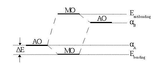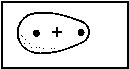
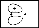
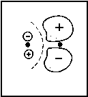
Fig. 1: In a heteronuclear molecule the bonding MO is closer to the more electronegative atom (A in the case shown here ). In the respective wave function Ψbonding, the atomic orbital ΦA is dominant. In contrast, the antibonding MO the original atomic orbital of the atom B (of lower electronegativity) are of similar energy and ΦB is dominant in Ψantibonding.

The larger the difference between α_A and α_B, the larger is the denominator in the fraction and, in consequence, the smaller is the splitting of the MO energy levels. These levels are shown in Fig. 1. With almost identical values of α_A and α_B, the approximation above is not applicable anymore, but recalling the previous chapter homonuclear molecules, we are well prepared to treat this case where we are approach the situation α_A = α_B.

To obtain the coefficients c_A and c_B that represent the weight of the single atomic orbitals, we introduce the obtained expression for E_bonding into equation (α_A - E) c_A + (β - ES) c_B = 0. Using again the approximation E ≈ a_A- ΔE or ΔE<<a_A we find:

^cA/c_B  =  ^{(β - a}A^S)/ΔE ^{= - [α}B ^{- a}A^]/[β - α_AS]

Coefficient c_A emerges when Ψ_bonding is normalized. In analogy, for the antibonding MO we recieve

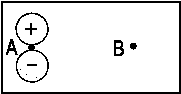
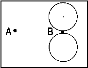
^cB/c_A =  ^{(β - a}B^S)/[α_B-α_A]

As a threedimensional plot, Fig. 2 illustrates a linear combination with differently weighted atomic wave functions. Φ_A is an 2p_z-, Φ_B is an 1s-orbital. The ratio c_B/c_A is 3/7.
 

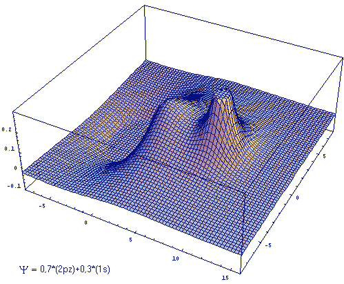
Fig .2: Example for the wave function that emerges from a linear, differently weighted combination of an 2pz and an 1s atomic orbital.

Fig. 3 shows a correlation diagram for a heteronuclear diatomic molecule (comp. homonuclear case). Just σ and π appear as the g-u-classification is only relevant for homonuclear diatomics. Fig. 4 qualitatively shows the distribution of the wave function's amplitude for the single atoms and the orbitals of an hypothetical united atom as the two extremes in this approach. The intermediate case between shall deliver an impression of the conditions in a molecule AB.
 

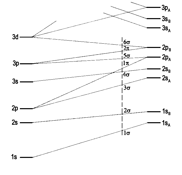Fig.3: Correlation diagram for a heteronuclear diatomic molekule (compare Fig. 1 Energy Levels in homonuclear molecules). Only σ and π molecular orbitals are of interest. The vertical dashed line represents the sequence of MO energies found in the Molecule NO (according to R.S. Mulliken, Rev. mod. Phys. 4, 1 (1932)).

1s		<=>		<=>		1sA
2s		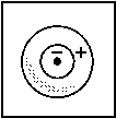<=>		<=>		1sB
2px		<=>		<=>		2pxA
3px		<=>		<=>		2pxB
	united atom		molecule		single atoms
Fig. 4: Examples of the correlation between orbitals of a united atom and the single atoms for a heteronuclear diatomic molecule. The atomic orbitals of the separate atoms on the right yield in one bonding and one antibonding combination one molecular orbital (in the middle) and, in the hypothetical case of an internuclear distance zero, atomic orbital (left). Pay attention to the case of the antibonding combination depicted in the last row. Here, an additional node appears and an AO with an increased quantum number (3px) is introduced.

 
 

Auf diesem Webangebot gilt die Datenschutzerklärung der TU Braunschweig mit Ausnahme der Abschnitte VI, VII und VIII.